In this post I will try to explain the overall structure as well as how I went about implementing the model described in the LittleBird[1] paper.
Intro
LittleBird is a sparse attention model proposed by Kakao Enterprise Corp. that improves on BigBird by reducing the memory footprint and improving the speed while maintaining accuracy. The model is a combination of BigBird's sliding window attention and LUNA pack and unpack attention with a custom bi-directional positional representation method based on ALiBi. As of 2022.03.08 the model sits at first place on the KorQuad 2.0 test set.
Let's begin by taking a look at the various formulas shown in the paper to get an idea of how one may go about implemnting the model.
In this post I focus almost exclusively on my implementation of the LittleBird model. For those curious about the training methods used the by authors, or the more theoretical aspects of the model, I recommend reading the paper.
Formulas
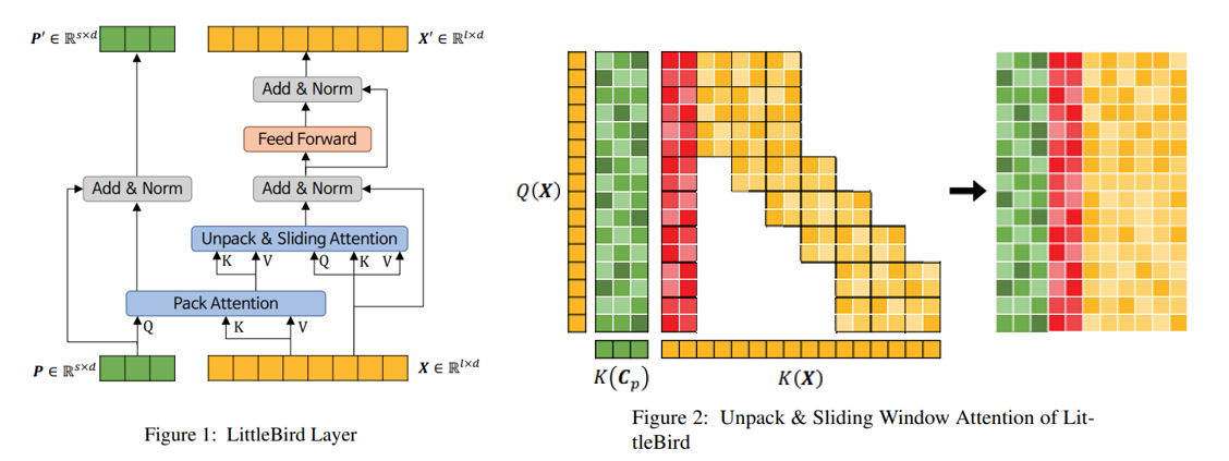
LittleBird Layer
where is the input sequence, and and 는 are the sequence length and embedding dimension respectively. is Pack Attention's projection matrix, and is the length of the packed sequence.
Attention
where is the row-wise concatenation of and , and refers to Unpack & Sliding Window Attention.
BiALiBi
where is the distance function for representing positional data for Pack Attention, and is all-ones matrix with size x . is the distance function, named BiALiBi by the authors, used to represent the positional information for LittleBird's Sliding Window Attention. , , are all trainable parameters.
Hyperparmaters
It's a good idea to know what the hyperparameters used in the model are, so I listed them in the table below. These will also be referenced in the various code samples below.
| variable | dtype | default value | description |
|---|---|---|---|
| seq_len | int | None | length of the input sequence |
| pack_len | int | None | length of the project matrix |
| d_model | int | 512 | embedding size |
| d_ff | int | 2048 | FeedForward layer size |
| num_attention_heads | int | 8 | - |
| num_heads | int | 8 | same as num_attention_heads |
| dropout_p | float | 0.1 | - |
| block_size | int | 64 | block size used for calculating USWAttention |
| window_size | int | 3 | window size used when calculating Sliding Window Attention |
LittleBirdLayer
I would like to focus on building the LittleBirdModel using a top-down approach starting with the LittleBirdLayer. As shown in the formula above, the layer is composed of three LayerNorms, a FeedForward layer, a MultiHeadAttention layer, and the USWAttn layer. This is pretty easy to implement and we can do so as shown below.
init
class LittleBirdLayer(nn.Module):
    def __init__(...) -> None:
        ...

        self.pack_attn = PackAttention(d_model, num_attention_heads)
        self.unpack_sliding_attn = UnpackSlidingWindowAttention(
            seq_len, pack_len, d_model, num_attention_heads, block_size
        )
        self.feed_forward = PositionwiseFeedForwardNetwork(d_model, d_ff, dropout_p)

        self.pack_attn_layer_norm = nn.LayerNorm(d_model)
        self.unpack_sliding_attn_layer_norm = nn.LayerNorm(d_model)
        self.ffn_layer_norm = nn.LayerNorm(d_model)
Forward
Since we have conveniently abstracted the work to their respective layers, we can implement the forward pass almost exactly as it is written in the formula above.
Our model will have multiple layers, so we need to return both and as we will pass them directly into the next layer as and .
    def forward(
        self,
        P: torch.Tensor,
        X: torch.Tensor,
        attention_mask: torch.Tensor
    ):
        Cp = self.pack_attn(P, X, attention_mask)
        P0 = self.pack_attn_layer_norm(Cp + P)

        Cx = self.unpack_sliding_attn(X, Cp, attention_mask)
        A = self.unpack_sliding_attn_layer_norm(Cx + X)

        X0 = self.ffn_layer_norm(self.feed_forward(A) + A)

        return P0, X0
Feed Forward
With transformers, it's common to add non-linearity to the model using a FeedForward layer. The usage of this particular class is shown in the code sample directly above.
Here we just implement the layer as described in the original transformer paper.
class PositionwiseFeedForwardNetwork(nn.Module):
    def __init__(...) -> None:
        super(PositionwiseFeedForwardNetwork, self).__init__()
        self.feed_forward = nn.Sequential(
            nn.Linear(d_model, d_ff),
            nn.Dropout(dropout_p),
            nn.ReLU(),
            nn.Linear(d_ff, d_model),
            nn.Dropout(dropout_p),
        )

    def forward(self, inputs: torch.Tensor) -> torch.Tensor:
        return self.feed_forward(inputs)
PackAttention
The pack part of Pack and Unpack Attention is the same as multihead attention from the original transformer model. We can just use the built-in Pytorch methods to impelement this is a few lines.
class PackAttention(nn.Module):
    def __init__(...):
        super(PackAttention, self).__init__()
        self.embed_dim = embed_dim
        self.num_heads = num_heads

        self.mha = nn.MultiheadAttention(
            embed_dim=self.embed_dim, num_heads=self.num_heads, batch_first=True
        )

    def forward(self, P: torch.Tensor, X: torch.Tensor, attention_mask: torch.Tensor):
        attn, _ = self.mha(P, X, X, attention_mask)
        return attn
USWAttention
Let us move on to implementing Unpack & Sliding Window Attention.
init
As shown in Figure 2 above, Unpack & Sliding Window Attention is composed of the Unpack Attention and Global + Sliding Window Attention. Additionally, the location information for each part is represented using a uniform distance matrix and BiALiBi respectively.
class UnpackSlidingWindowAttention(nn.Module):
    def __init__(...):
        super(UnpackSlidingWindowAttention, self).__init__()

        # Hyperparameters
        self.attn_head_size = int(dim / num_attention_heads)
        self.num_attention_heads = num_attention_heads
        self.block_size = block_size
        self.seq_len = seq_len
        self.pack_len = pack_len

        # QKV linear transformation layers
        self.Q = nn.Linear(dim, self.attn_head_size * num_attention_heads)
        self.K = nn.Linear(dim, self.attn_head_size * num_attention_heads)
        self.V = nn.Linear(dim, self.attn_head_size * num_attention_heads)

        # location information
        self.bialibi = BidirectionalALiBi(
            self.num_attention_heads, self.seq_len
        )
        self.uniform_dist_mat = UniformDistanceMatrix(
            self.num_attention_heads, self.block_size, self.seq_len, self.pack_len
        )


        self.register_buffer("middle_band_distance_indicies", None, persistent=False)
Linear Transformations
We start by calculating the scaling factor , where , since we are also doing multihead attention.
Next we perform the linear transformations of into , , , and into and .
We follow up by splitting the transformations into , and transposing the matrix such that the last two layers correspond to and .
    def forward(self, X, Cp, ...)

        ...

        rsqrt_d = 1 / math.sqrt(self.attn_head_size)

        batch_size, seq_len, dim = X.shape

        query = transpose_for_scores(
            self.Q(X), self.num_attention_heads, self.attn_head_size
        )  # bsz, head, seq_len, head_dim
        key_x = transpose_for_scores(
            self.K(X), self.num_attention_heads, self.attn_head_size
        )  # bsz, head, seq_len, head_dim
        value_x = transpose_for_scores(
            self.V(X), self.num_attention_heads, self.attn_head_size
        )  # bsz, head, seq_len, head_dim

        key_Cp = transpose_for_scores(
            self.K(Cp), self.num_attention_heads, self.attn_head_size
        )  # bsz, head, pack_len, head_dim
        value_Cp = transpose_for_scores(
            self.V(Cp), self.num_attention_heads, self.attn_head_size
        )  # bsz, head, pack_len, head_dim

        ...
See the impelmentation for transpose_for_scores below in the Utility Functions section.
Unpack Attention
Next we will move on to calculating the Unpack Attention part of Unpack & Sliding Window Attention.
In typical self-attention, one would first calculate the attention scores between the key and query vectors, scale them, and multiply them by the value vectors to get the context vector. On the other hand, USW Attention calculates the attention scores and contexts using the concatenation of and , and and .
We can achieve this by calculating the sliding attention and unpack attention separately and adding them together in the end.
Since the order isn't super important, we will start with unpack attention.
Code
Note the line key_cp_attn[:] -= Dp. Here we are apply the uniform distance matrix to the attention scores before calculating the context.
    # Step 1 calculate the attention scores for the packed data
    key_cp_attn = torch.matmul(query, key_Cp.transpose(2, 3))
    key_cp_attn = key_cp_attn * rsqrt_d
    key_cp_attn[:] -= Dp
    key_cp_attn = F.softmax(key_cp_attn, dim=-1)  # bsz, heads, seq_len, pack_len

    packed_context = torch_bmm_nd(key_cp_attn, value_Cp, ndim=4)
Global + Sliding Window
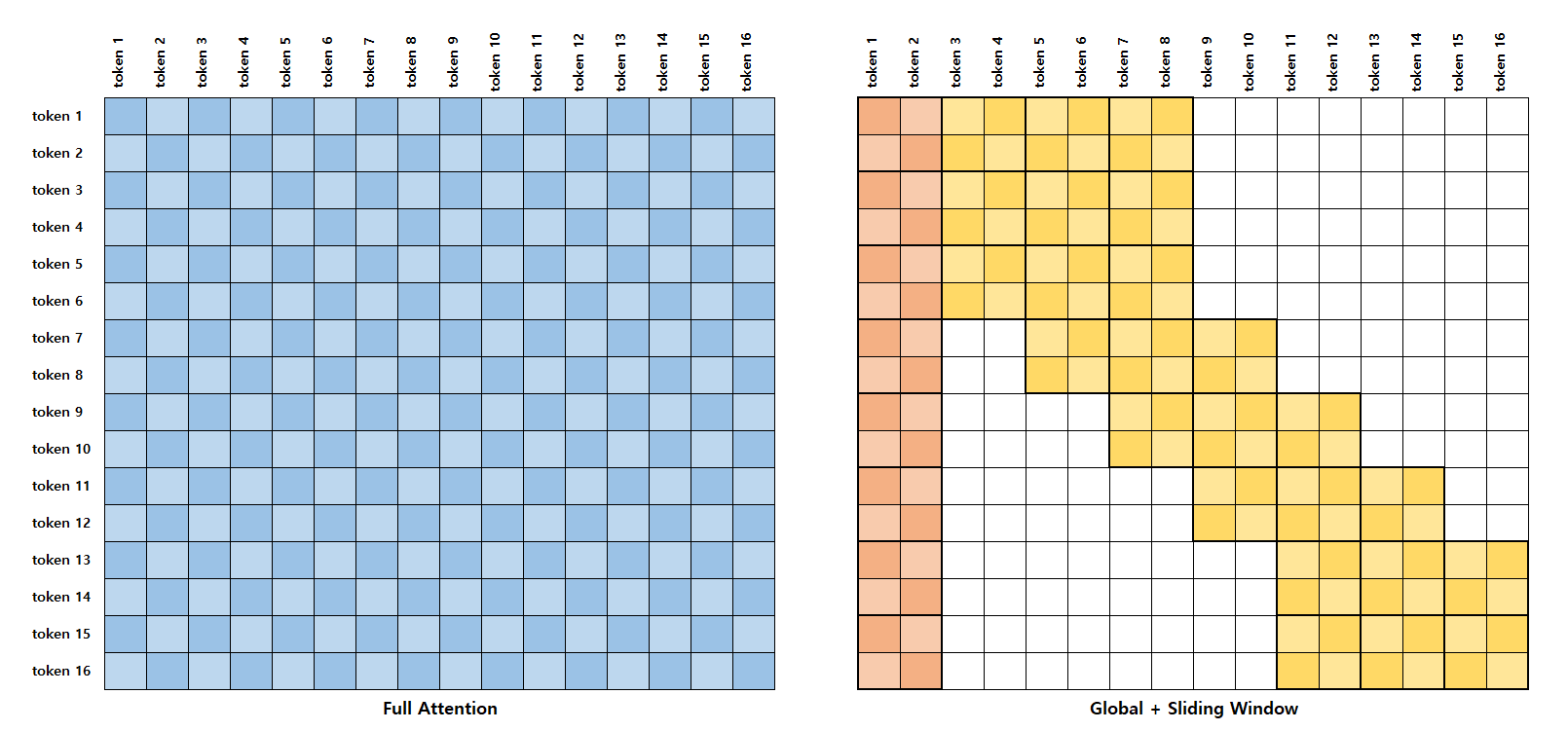
Figure 3: Full Attention과 Global + Sliding Window Attention 비교
Due to the quadratic time complexity of typical self-attention, working with sequence lengths longer than 512 becomes computationally expensive, whereas using a sparse attention method, like the one proposed in LittleBird, one can reduce the time complexity allowing for significantly longer input sequences.
The image above depicts how this would look in comparison to typical self-attention. The white squares represent attention scores that we do not calculate.
The authors mention that with a small enough and the time complexity for LittleBird's attention can be considered to have a linear time complexity wrt . More specifically, compared to self-attention's .
Unfortunately, as it is well known that performing sparse multiplications cannot be efficiently implemented on the GPU, the authors of the BigBird paper proposed blocking the sets of query and keys together and performing the attention calculating between these blocks instead. This will serve as the basis for which we will calculate LittleBird's global + sliding window attention.
Blockify the input

Figure 4: blockify example with a seq_len of 512 and a block_size of 64
Blockifying the sequence is as simple as calling the view method on the vectors as shown below.
query_block = query.view(
    batch_size,
    self.num_attention_heads,
    seq_len // self.block_size,
    self.block_size,
    -1,
)
key_x_block = key_x.view(
    batch_size,
    self.num_attention_heads,
    seq_len // self.block_size,
    self.block_size,
    -1,
)
value_x_block = value_x.view(
    batch_size,
    self.num_attention_heads,
    seq_len // self.block_size,
    self.block_size,
    -1,
)
First two rows
We calculate the attention scores in three steps: the first two rows, the middle band, and the last row.
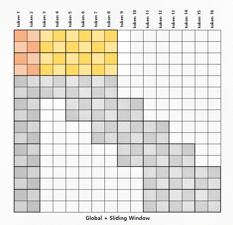
Figure 4: Attention for the first two rows
We calculate the first two and last rows separately from the middle rows because we want to preserve the order of the blocks in which we calculate attention. This will become more clear in the following sections.
Code
Note that the dimensions for the vectors at this point are:
batch_size, attn_heads, num_blocks, block_size, head_dim = key_x_block.shape
We first transpose the key, value vectors such that the first 4 blocks are grouped together, and we transpose the query such that the first two blocks are grouped together.
# Step 2.1. process the first two rows
first_two_rows_key_matrix = torch.cat(
    [
        key_x_block[:, :, 0],
        key_x_block[:, :, 1],
        key_x_block[:, :, 2],
        key_x_block[:, :, 3],
    ],
    dim=2,
)
first_two_rows_value_matrix = torch.cat(
    [
        value_x_block[:, :, 0],
        value_x_block[:, :, 1],
        value_x_block[:, :, 2],
        value_x_block[:, :, 3],
    ],
    dim=2,
)

first_two_query_blocks = torch.cat(
    [query_block[:, :, 0], query_block[:, :, 1]], dim=2
)
Next we:
- calculate the attention scores with the key and query vectors
- scale the attention scores
- subtract the biases from the BiALiBi distance matrix
- take into account the attention mask
- softmax
- and finally calculate the context with the value vectors
first_two_rows_attn = torch_bmm_nd_transpose(
    first_two_query_blocks, first_two_rows_key_matrix, ndim=4
)
first_two_rows_attn *= rsqrt_d
first_two_rows_attn -= D[:, : self.block_size * 2, : self.block_size * 4]
first_two_rows_attn += (1.0 - self.mask_v[:, :, :self.block_size * 2, :self.block_size * 4]) * attn_penalty
first_two_rows_attn = F.softmax(first_two_rows_attn, dim=-1)

first_two_rows_context = torch_bmm_nd(
    first_two_rows_attn, first_two_rows_value_matrix, ndim=4
)
In the final step, we will concatenate the results from the first two rows, the middle band, and the last two rows to get a final context vector. We will concatenate on the block dimension and as such need to reshape the context vector.
_, __, ftr_3d, ftr_4d = first_two_rows_context.shape
first_two_rows_context = first_two_rows_context.view(
    batch_size, self.num_attention_heads, 2, ftr_3d // 2, ftr_4d
)  # bsz, heads, 2(blocks), block_size, block_size*4
Sliding Window (Middle Band)
In this section, we use the techniques described in the BigBird paper to calculate the attention for the middle band.
I also recommend reading the explanation in the BigBird paper or HuggingFace blog[5] to supplement my own and maybe fill in any gaps!
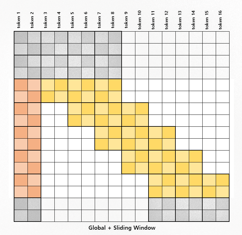
Figure 4: Attention for the middle band
How it Works
We take the blocked key vectors and copy them twice with the elements shifted once to the left and once to the right. If we then multiply the query vectors by the 3 shifted vectors, we can cover all of the sliding tokens.
This works because we're multiplying along the blocked dimension. Consider the image below. Multiplying along the block dimension between the keys and query would give us the attention scores for the elements in those blocks only.
When multiplying the query with the unshifted keys, we get the attention scores for the blocks on the diagnol. If we shift the values to the right and left, and do the same multiplication operation, we get the scores for the blocks just left and right of the diagnol.
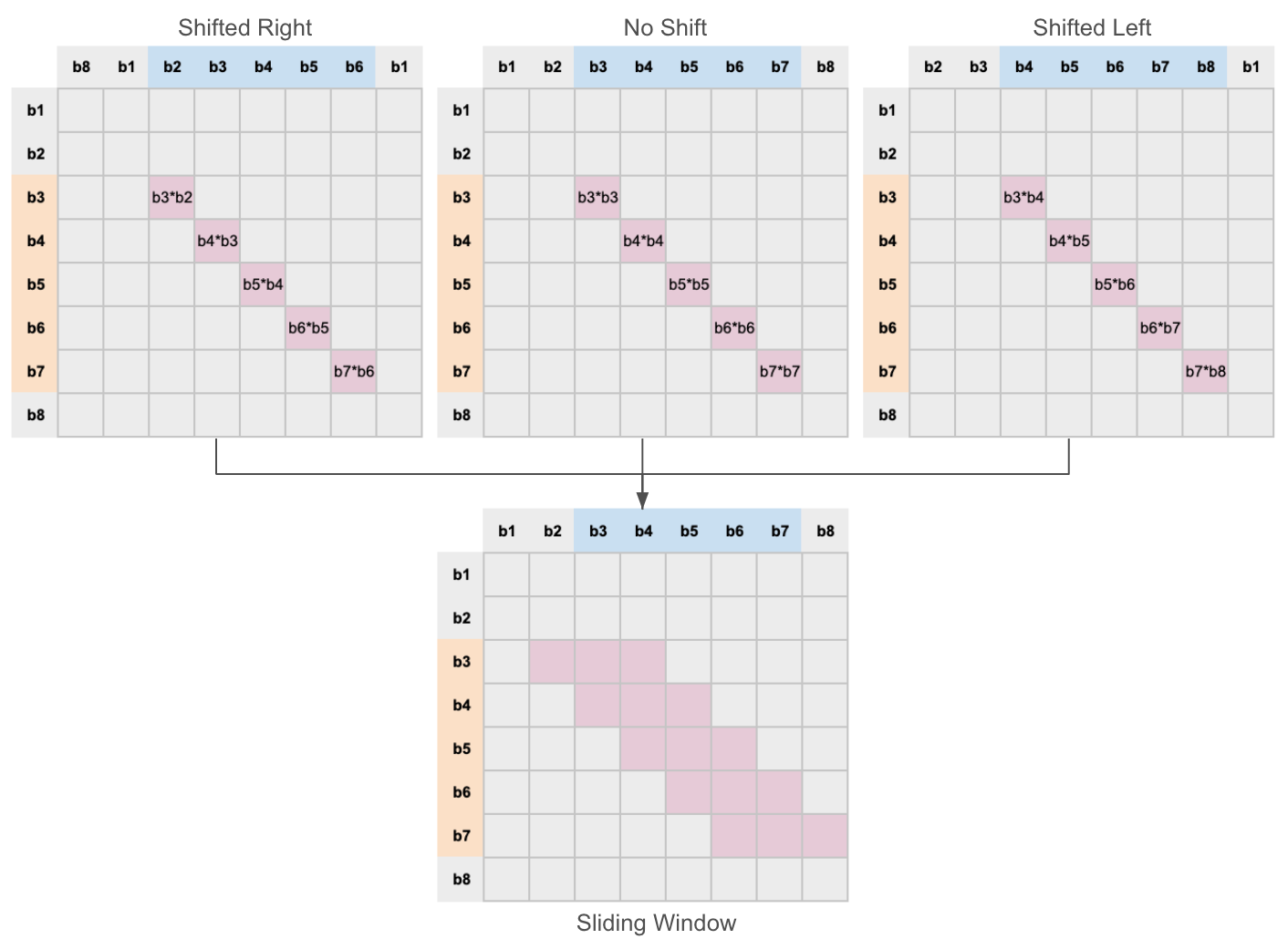
Figure 4: The three steps that go into calculating the sliding window attention
Sliding Window implementation
# step 2.2 calculate the middle part of the matrix
# the trick described in the bigbird paper is used

middle_band_key_matrix = torch.cat(
    [
        key_x_block[:, :, 1:-2],  # roll back one
        key_x_block[:, :, 2:-1],
        key_x_block[:, :, 3:],  # roll forward one
    ],
    dim=3,
)
middle_band_value_matrix = torch.cat(
    [
        value_x_block[:, :, 1:-2],  # roll back one
        value_x_block[:, :, 2:-1],
        value_x_block[:, :, 3:],  # roll forward one
    ],
    dim=3,
)


# get the diagnol
middle_band_sliding = torch_bmm_nd_transpose(
    query_block[:, :, 2:-1], middle_band_key_matrix, ndim=5
)
middle_band_sliding += (1.0 - self.band_mask) * attn_penalty
Global Attention Implementation
LittleBird also calculates a global attention by attending the first block to every other token in the sequence. This is represented by the orange strip in the Global + Sliding Window image above. We can calculate this separately and concatenate it with the result of the sliding window operation.
# get the global
middle_band_global = torch.einsum(
    "bhlqd,bhkd->bhlqk", query_block[:, :, 2:-1], key_x_block[:, :, 0]
)
middle_band_global += (1.0 - self.mask_block[:,2:-1,:].unsqueeze(3)) * attn_penalty

middle_band_attn = torch.cat([middle_band_global, middle_band_sliding], dim=-1)
middle_band_attn *= rsqrt_d
middle_band_attn -= self.get_middle_band_distances(D)
middle_band_attn = F.softmax(middle_band_attn, dim=-1)

middle_band_context = torch.einsum(
    "bhlqk,bhkd->bhlqd",
    middle_band_attn[:, :, :, :, : self.block_size],
    value_x_block[:, :, 0],
)
middle_band_context += torch_bmm_nd(
    middle_band_attn[:, :, :, :, self.block_size : 4 * self.block_size],
    middle_band_value_matrix,
    ndim=5,
)
Last Row
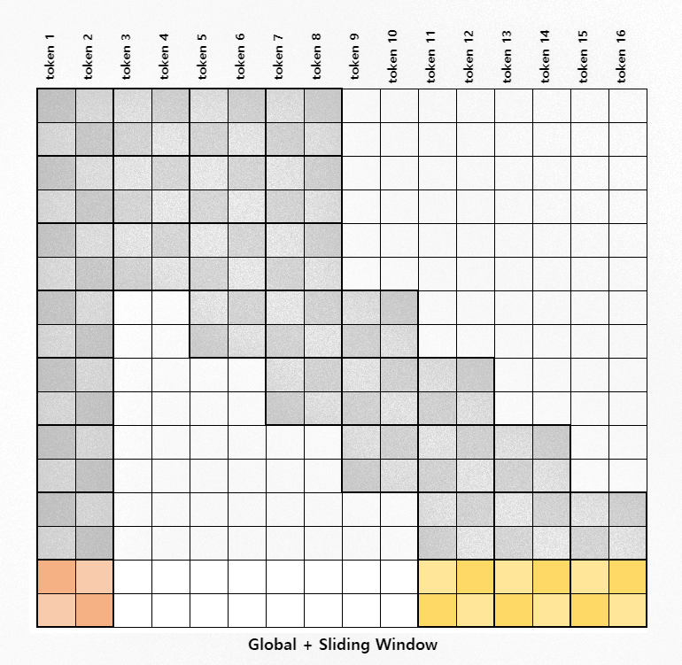
Figure 4: Attention for the last row
The last row is done similarly to the first two rows but we use the first block and the last three blocks, as opposed to the first four blocks, for the key and value vectors.
# calcualte the last row
last_row_key_matrix = torch.cat(
    [
        key_x_block[:, :, 0],
        key_x_block[:, :, -3],
        key_x_block[:, :, -2],
        key_x_block[:, :, -1],
    ],
    dim=2,
)
last_row_value_matrix = torch.cat(
    [
        value_x_block[:, :, 0],
        value_x_block[:, :, -3],
        value_x_block[:, :, -2],
        value_x_block[:, :, -1],
    ],
    dim=2,
)

last_row_attn = torch_bmm_nd_transpose(
    query_block[:, :, -1], last_row_key_matrix, ndim=4
)
last_row_attn *= rsqrt_d
last_row_attn -= D[:, -self.block_size :, -self.block_size * 4 :]
last_row_attn = F.softmax(last_row_attn, dim=-1)

last_row_context = torch_bmm_nd(last_row_attn, last_row_value_matrix, ndim=4)
last_row_context.unsqueeze_(2)
Bringing everything together
To finish up, we concatenate the contexts from the first two rows, the middle band, and the final row; do some reshaping; add the packed and sliding window context; and reshape the final context vector.
context_layer = torch.cat(
    [first_two_rows_context, middle_band_context, last_row_context], dim=2
)
context_layer = context_layer.view(
    (batch_size, self.num_attention_heads, seq_len, -1)
)

Cx = context_layer + packed_context
Cx = Cx.view(
    batch_size, seq_len, self.num_attention_heads * self.attn_head_size
) * self.mask_v.squeeze(1)

return Cx
BiALiBi
We can achieve the BiALiBi matrix by breaking it down into largely three steps. We initialize a vector representing the absolute distances from the diagnol; calculate masks filled with the trainable γ, β, and α values; and finish by performing elementwise multiplciation between the distance vector and the masks.
Step 1. Create the base distance matrix
row_i = torch.arange(self.seq_len, dtype=torch.float32)
col_i = torch.arange(self.seq_len, dtype=torch.float32).unsqueeze(-1)
distances = (row_i - col_i).abs()
distances

tensor([[0, 1, 2, 3, 4, 5],
        [1, 0, 1, 2, 3, 4],
        [2, 1, 0, 1, 2, 3],
        [3, 2, 1, 0, 1, 2],
        [4, 3, 2, 1, 0, 1],
        [5, 4, 3, 2, 1, 0]], dtype=torch.int32)
Step 2. Create the gamma(γ) and beta(β) masks
gamma_mask = torch.triu(torch.ones_like(self.distances), diagonal=1)
gamma_mask *= self.gamma.view(-1, 1, 1)
gamma_mask

tensor([[[0.0000, 0.4540, 0.4540, 0.4540, 0.4540, 0.4540],
         [0.0000, 0.0000, 0.4540, 0.4540, 0.4540, 0.4540],
         [0.0000, 0.0000, 0.0000, 0.4540, 0.4540, 0.4540],
         [0.0000, 0.0000, 0.0000, 0.0000, 0.4540, 0.4540],
         [0.0000, 0.0000, 0.0000, 0.0000, 0.0000, 0.4540],
         [0.0000, 0.0000, 0.0000, 0.0000, 0.0000, 0.0000]]],
       grad_fn=<MulBackward0>)
beta_mask = torch.tril(torch.ones_like(self.distances), diagonal=-1)
beta_mask *= self.beta.view(-1, 1, 1)
beta_mask

tensor([[[0.0000, 0.0000, 0.0000, 0.0000, 0.0000, 0.0000],
         [0.9392, 0.0000, 0.0000, 0.0000, 0.0000, 0.0000],
         [0.9392, 0.9392, 0.0000, 0.0000, 0.0000, 0.0000],
         [0.9392, 0.9392, 0.9392, 0.0000, 0.0000, 0.0000],
         [0.9392, 0.9392, 0.9392, 0.9392, 0.0000, 0.0000],
         [0.9392, 0.9392, 0.9392, 0.9392, 0.9392, 0.0000]]],
       grad_fn=<MulBackward0>)
Step 3. Add the masks and insert the alpha(α) parameter.
mask = beta_mask + gamma_mask

# step 4: set the alphas
mask[:, 0, :] = 1.0
mask[:, :, 0] = 1.0
mask[:, 1:, 0] *= self.alpha.unsqueeze(1)
mask[:, 0, 1:] *= self.alpha.unsqueeze(1)
mask[:, 0, 0] *= 0.0

tensor([[[0.0000, 0.7959, 0.7959, 0.7959, 0.7959, 0.7959],
         [0.7959, 0.0000, 0.4540, 0.4540, 0.4540, 0.4540],
         [0.7959, 0.9392, 0.0000, 0.4540, 0.4540, 0.4540],
         [0.7959, 0.9392, 0.9392, 0.0000, 0.4540, 0.4540],
         [0.7959, 0.9392, 0.9392, 0.9392, 0.0000, 0.4540],
         [0.7959, 0.9392, 0.9392, 0.9392, 0.9392, 0.0000]]],
       grad_fn=<CopySlices>)
Now we can finish off by just multiplying the base distance matrix with the mask.
self.distances * mask

tensor([[[0.0000, 0.2621, 0.5243, 0.7864, 1.0486, 1.3107],
         [0.2621, 0.0000, 0.6620, 1.3239, 1.9859, 2.6478],
         [0.5243, 0.4262, 0.0000, 0.6620, 1.3239, 1.9859],
         [0.7864, 0.8524, 0.4262, 0.0000, 0.6620, 1.3239],
         [1.0486, 1.2787, 0.8524, 0.4262, 0.0000, 0.6620],
         [1.3107, 1.7049, 1.2787, 0.8524, 0.4262, 0.0000]]],
       grad_fn=<MulBackward0>)
Utility functions
Below are functions borrowed and slightly modified from HuggingFace's implementation of BigBird.
def torch_bmm_nd_transpose(inp_1, inp_2, ndim=None):
    """Fast nd matrix multiplication with transpose"""
    # faster replacement of torch.einsum (bhqd,bhkd->bhqk)
    return torch.bmm(
        inp_1.reshape((-1,) + inp_1.shape[-2:]),
        inp_2.reshape((-1,) + inp_2.shape[-2:]).transpose(1, 2),
    ).view(inp_1.shape[: ndim - 2] + (inp_1.shape[ndim - 2], inp_2.shape[ndim - 2]))


def torch_bmm_nd(inp_1, inp_2, ndim=None):
    """Fast nd matrix multiplication"""
    # faster replacement of torch.einsum ("bhqk,bhkd->bhqd")
    return torch.bmm(
        inp_1.reshape((-1,) + inp_1.shape[-2:]), inp_2.reshape((-1,) + inp_2.shape[-2:])
    ).view(inp_1.shape[: ndim - 2] + (inp_1.shape[ndim - 2], inp_2.shape[ndim - 1]))


def transpose_for_scores(x, num_attn_head, attn_head_size):
    new_x_shape = x.size()[:-1] + (num_attn_head, attn_head_size)
    x = x.view(*new_x_shape)
    return x.permute(0, 2, 1, 3)
Additional Info
Thank you for reading.
You may view the full source code on Github.
If you have any comments regarding this explanation or perhaps I have any mistakes in my impelmentation, please feel free to open an issue on the Github repository above! 😊
References
- [1] LittleBird: Efficient Faster & Longer Transformer for Question Answering
- [2] Big Bird: Transformers for Longer Sequences
- [3] Luna: Linear Unified Nested Attention
- [4] Train Short, Test Long: Attention with Linear Biases Enables Input Length Extrapolation
- [5] Understanding BigBird's Block Sparse Attention